Final Report

Implementing parallelism using different architectures : Shashank Ojha and Kylee Santos

Final Report

Summary

We created optimized implementations of gradient descent on both GPU and multi-core CPU platforms, and perform a detailed analysis of both systems’ performance characteristics. The GPU implementation was done using CUDA, whereas the multi-core CPU implementation was done with OpenMP.

Background

Gradient descent is a technique used to find a minimum using numerical analysis in times where directly computing the minimum analytically is too hard or even infeasible. The idea behind the algorithm is simple. At any given point in time, you determine the effect of modifying your input variable on the cost function you are trying to minimize. In the one dimensional case, if increasing the value of your input decreases your cost function, then you can increase the value of your input by a small step to get you closer to the minimum cost. Generalizing to higher dimensions, the gradient tells you the direction of the greatest increase on your cost function, so you can move the input in the opposite direction to hopefully decrease the value of the cost function.

Building on top of this idea, there are two kinds of gradient descent methods. One is called batch gradient descent (BGD) and the other is stochastic gradient descent (SGD). Let’s discuss both. We can imagine we have some regression problem where we are trying to estimate some function f(x). We are given n labeled data points of the form (xi, f(xi)). Our job is to find some estimator, gw(x) of the desired function such that we minimize the mean squared error, J(w) = 1/n Sum[f(xi) -gw(xi)]^2. Formally, we let w be a vector representing all the parameters of of the function gw(x). Our goal is to find the optimal w that minimizes our cost function. Now in order to find the true gradient of our cost function, we would need to plug in all our points. This is what is known as batch gradient descent. The update step looks like the following: wi+1 = wi - ∇J(w)

Here, we do the above for each element of our vector w and move with some small step size η. If n is large, however, this computation can be very expensive especially since at each time step we only make a small modification. Thus, it does not always make sense to do such a heavy computation to make a tiny step forward. In contrast, stochastic gradient descent chooses a random data point to determine the gradient. This gradient is much noisier since it doesn’t have the whole picture, but it can greatly speed-up performance. In most cases, it is best to start with stochastic gradient descent, but then eventually switch to batch for fine-grained movement.

The last important detail to discuss is the concept of local and global minima. When the cost function we are trying to minimize is convex, any local minima will be equal to the global minima by definition. However, for non-convex functions, we might stumble across a local minima as opposed to a global minima. Consider the following graphic take from Howie Choset’s Robot Kinematics and Dynamics class.

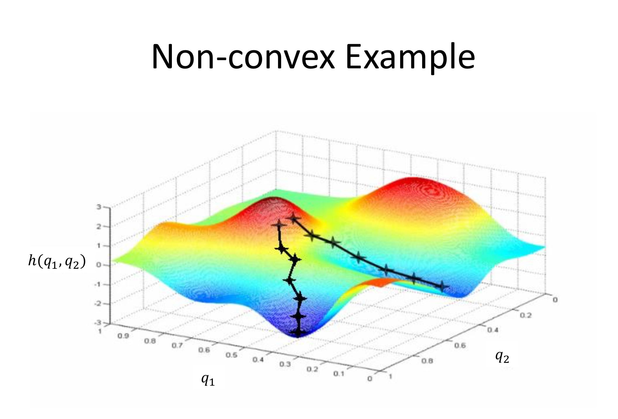
As you might observe, the initial position start state may affect our answer when performing gradient descent. This is because the gradient is different at each point and thus starting at a different point may take us in a different direction. With respect to stochastic and batch gradient descent, stochastic gradient has the property that it might jump out of local minima because it has a random aspect to it that makes the gradient more noisy. This has a variety of applications in machine learning where we are working with large data sets and gradient descent becomes very computationally intensive.

In the context of this project, we came across some papers that were able to optimize gradient descent with the use of more parallel power. While gradient descent is generally a sequential algorithm, it seems like the use of parallelism can speed up the convergence rate of gradient descent and thus allow us to reach a much better approximation of the optimal value in the same wall clock time. This is due to the fact that multiple processing units allows us to extract more information from our data set per clock cycle and thus allows us to make a more accurate update towards the optimal. The papers that inspired us to try this are linked in the references section.

Approach

There were two aspects to the project (1) optimizing gradient descent on CPUs on Xeon Phi machines by making use of their fast clock speed and (2) optimizing gradient descent on NVIDIA GeForce GTX 1080 GPUs by making use of the large number of threads they have. We present our approaches on each of the architectures below. In both cases, we performed gradient descent on a regression problem, where our target function was f(x) = ax3 + bx2 + cx +d. Thus, the vector we tried to minimize consisted of the function’s coefficients, namely w=<a, b, c, d>. Our cost function was J(w) = 1/n Sum[f(xi) -gw(xi)]^2.

Xeon Phi Machines

For the Xeon Phi Machines, our initial approach was to use the multiple processing units to compute the gradients quicker. Note that stochastic gradient descent chooses a point from our data set uniformly at random, computes the gradient, and performs the update. The first downside to this algorithm is that it is entirely serial since updates must occur sequentially. Therefore, for this project, we looked to increase the performance of our program by computing a more accurate estimate in a fixed amount of time. In terms of accuracy, the issue with stochastic gradient descent is that each update has a high variance because it is only using information from one point as opposed to all the data like batch gradient descent does. Thus, we hypothesized that in the time we compute the gradient of one point, we can actually compute t gradients in parallel where t is the number of threads. Each thread can compute the gradient of a point and this will allow us to use information from t points at a time, as opposed to just once and thus allowing the steps to be more accurate. This approach, however, falls short due to the high communication required to average the gradients of the t threads together. The computation needed to compute the gradient at a point is dominated by the time needed to communicate. One of our proposed solutions for this problem of poor arithmetic intensity was to simply increase the amount of computation that each thread performed before they communicated. In other words, instead of computing the gradient after looking at a single point, each thread can compute the gradient based on k points in order to make a more informed step towards the minimum and to decrease the communication-to-computation ratio. These approaches deviated from the normal stochastic implementation, since the threads collectively compute a mini-batch of the points before updating the global estimate. Furthermore, if all of the points were partitioned evenly and disjointly, this approach would actually parallelize batch gradient descent. This was one approach we coded up using OpenMP. Throughout the paper, we reference this approach as Stochastic Gradient Descent with K Samples.

Our second parallel approach was taken from the first paper under references. Despite our efforts to increase the arithmetic intensity in the design outlined above, all the threads would still have to communicate after each iteration, which slowed down the code drastically. The aforementioned paper introduces a very simple strategy that completely absolves the need for communication until the end. We do this by running the SGD completely independently on each thread for some large number of steps and then averaging the parameters. This does surprising well as can be seen in the results section. The correctness performance of this approach differs from the previous one because we only aggregate the resulting parameters of each thread at the very end. After each iteration of this approach, a thread cannot benefit from the results of the others since there is no communication during the descent. However, it can still run for less total iterations compared to the sequential implementation because the less accurate results of the individual threads are ultimately averaged out to an estimate that is closer to convergence. Throughout the paper, we reference this approach as Stochastic Gradient Descent Per Thread.

One huge problem with SGD is that its memory access is random. With larger and larger datasets, it’s almost certain you will get a cache miss when you randomly pick and access a point from your dataset. One way to alleviate this problem is to shuffle the data once on each thread randomly and then each thread can traverse its sequence of points in their respective order, which largely reduces the number of cache misses during descent. For a single iteration, shuffling the data once at the start of each thread’s computation is expensive for the same reason as the last approach: random memory access. However, after many iterations, we are able to see a noticeable speedup in the code, provided that we reuse the same initially shuffled order every time. Instead of randomly accessing points in each iteration causing cache misses at nearly every access, this new approach ultimately requires one expensive shuffle at the beginning, but every iteration of SGD updates is dramatically faster due to spatial locality. We were able to speed up the code by more than 40x in one case with this optimization. This speedup comes with a small caveat though. The first pass of the sequence of points for each thread is somewhat similar to our other approaches for stochastic gradient descent because the points were randomly shuffled. So, traversing them is similar to randomly sampling without replacement. However, all subsequent passes of the data must traverse the same sequence in order to take advantage of locality. Thus, we don’t have a perfectly random selection of data as described by the original stochastic gradient descent algorithm, but we found this did not slow down our convergence rate. Throughout the paper, we reference this approach as Stochastic Gradient Descent by Epoch.

NVIDIA GeForce GTX 1080 GPU

We implemented all of the designs described above in CUDA as well in order to compare their performances. Additionally, we also implemented two other strategies that we thought would fit better for this Nvidia GPU architecture. The first strategy is a hybrid of the two approaches described in the Xeon Phi section. Given the two layers of parallelism in GPU namely blocks and threads, we thought we could use the idea of running different independent gradient descents at the block level and mini-batch gradient descent using shared memory at the thread level. Each thread would sample k points and at the end of each iteration, each block would update its gradient by averaging only its own threads’ estimates. After all the iterations are complete, the blocks would average their estimates of the parameters w to provide a final estimate. Throughout the paper, we reference this approach as Stochastic Gradient Descent By Block.

The second approach was inspired from the paper as well. In this design, we again ran SGD for a fixed number of steps on each thread, but each thread did not have access to all the data. The entire dataset would first be randomly partitioned among the t threads launched. With their respective subset of the data, each thread would shuffle its subset at the start of each iteration and then perform a sequential pass over it, updating the gradient at each point. Thus, each thread computed an estimate for their subset of the data, and the estimates are aggregated at the end to produce a final prediction of the parameters. In this design, however, there is a tradeoff between speed and performance, which we analyzed in detail later in the results section. Throughout the paper, we reference this approach as Stochastic Gradient Descent With Partition.

Results

We did our regression analysis on two datasets. Both of the datasets were from the University of California Irvine Machine Learning Repository. The first dataset was called the Combined Cycle Power Plant Data Set. It consisted of 9568 data points. From the dataset, we used the exhaust vacuum (V) attribute as x-coordinate and the average temperature (AT) attribute as the y-coordinate. The second data set was called the News Popularity in Multiple Social Media Platforms Data Set and consisted of 39644 data points. We used the Global Subjectivity attribute as the x-coordinate and the N Tokens Content as the y-coordinate. The features used were taken arbitrarily such that the cubic regression problem was relatively interesting.

We used R to visualize the data and find the reference parameters/mean-squared-error for each of the datasets. For the Power Plant data set, the reference polynomial was y = -0.77921x3 -91.231x2 + 615.29824x +19.65123 with a mean-squared-error of 15.09505. For the News Popularity data set, the reference polynomial was y = -6881.84x3 -20852.72x2 + 11995.1x + 546.51 with a mean-squared-error of 206144.2.

Batch Gradient Descent

We first started with some baseline measurements on batch gradient descent. We expected to see clear speedup here because batch gradient descent is a perfect parallel problem. If we have n points and t threads, then we can perform an update in O(n/t + t) time as opposed to the sequential O(n) time algorithm. As we can see from the plot below, this problem scales with the number of threads matching our theoretical result.

Figure 1: Plot of mean-squared-error over time for batch gradient descent using T = {1, 2, 4, 8, 16, 32, 64} threads run on Xeon Phi.

Stochastic Gradient Descent with K samples

The next design we implemented was stochastic gradient descent, but we varied how many points we sampled at a time before making an update. We generated two plots: one that varied k on just 1 thread, where k is the number of samples per update, and the other on 16 threads. The two plots are below.

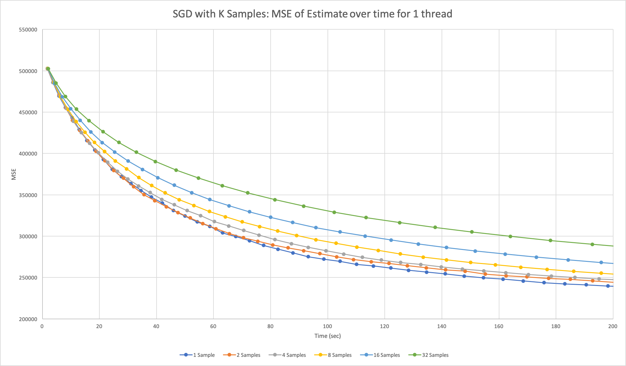
Figure 2: Plot of mean-squared-error over time for stochastic gradient descent using k = {1, 2, 4, 8, 16, 32} samples at a time on 1 thread run on Xeon Phi.

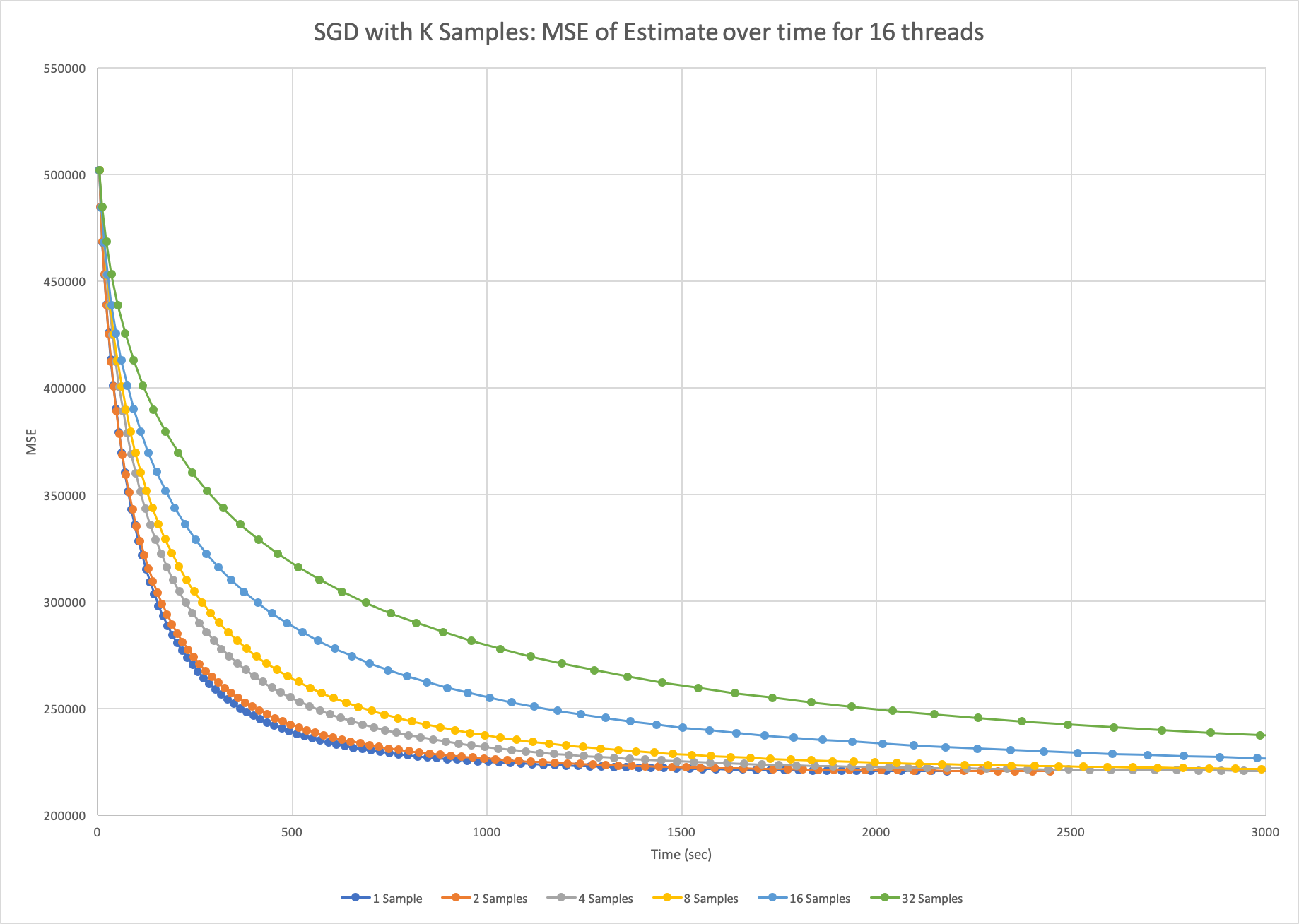
Figure 3: Plot of mean-squared-error over time for stochastic gradient descent using k = {1, 2, 4, 8, 16, 32} samples at a time on 16 threads run on Xeon Phi.

As we can see, sampling more points at a time doesn’t actually help us converge faster. This is an expected result because there is not that much information gain between 1 and 32 points when the data set is so large, but each update is 32 times slower. Of course, our plots don’t indicate that sampling a single point is 32 times faster than sampling 32 points because we do expect to make a more accurate step, but the cost of that additional information outweighs the benefits. From the second plot, we can see that adding parallelism here actually slows down the computations even more. The n threads would average their results to compute the global estimate after each iteration, introducing a communication overhead that caused a 10x slowdown in our program. We were able to time this piece of communication at each step to support our hypothesis for the cause of the program’s slowdown.

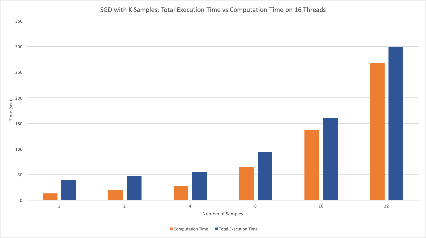
Figure 4: Graph of total execution time and computation time when running SGD with 16 threads and k samples for k = {1, 2, 4, 8, 16, 32}.

Stochastic Gradient Descent Per Thread

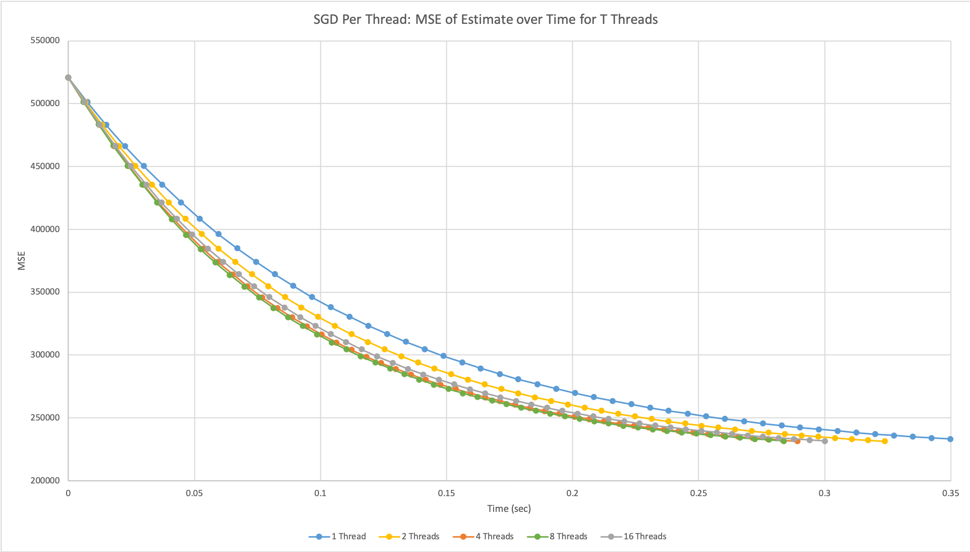
Figure 5: Plot of mean-squared-error over time using the SGD per thread design with T = {1, 2, 4, 8, 16} threads run on NVIDIA GeForce GTX 1080 GPU.

This code was implemented on both CPUs and GPUs, but the graph is from the GPUs because we were able to test how this approach scaled with more threads to the max. We were only able to measure time on the device in terms of clock cycles, but we were able to find the specs of the NVIDIA GeForce GTX 1080 GPU and used its clock rate to convert clock cycles to seconds. From looking at the axis of the graph, we can already see that this implementation runs significantly faster than even our fastest parallelized batch code. Comparing the behaviors of using different threads, we can see that our results are consistent with our reference paper. As we increased the number of threads (or independent SGD calls), we were able to see an increase in performance, more specifically, the program was able to converge to a near-optimal MSE faster. This behavior generally scales with the number of threads used; however, it is evident that with too many threads the performance begins to plateau, which can also be seen in the paper. We believe that this is because the estimates are ultimately still independently drawn from the same distribution and after a certain number of results, we will have enough points to represent the distribution and find its mean. Therefore, sampling even more points than that will not have a noticeable increase in result accuracy.

Stochastic Gradient Descent over Epochs

Here we use the number of epochs run to analyze the algorithm’s convergence. This is because this algorithm by nature does not require any communication, but the act of calculating the MSE from the separate estimates on each thread at a certain point in time requires communication and affects the runtime of the algorithm itself. The time taken to run an Epoch on each thread is the same however. Thus, we graph the MSE vs. Number of Epochs.

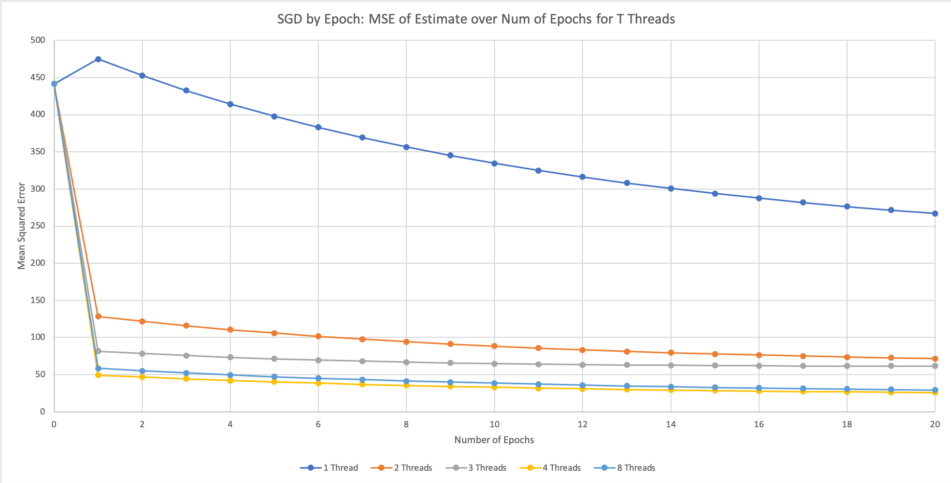
Figure 6: Plot of mean-squared-error over number of epochs using alternative SGD design with T = {1, 2, 3, 4, 8} threads run on Xeon Phi.

This plot is similar to the previous approach in that the parallelism comes from running SGD independently for each thread and averaging the results at the end. However, the figure above uses the alternative implementation of SGD using epochs. The first thing to note is that we had to use the first data set for these plots. This is because the difference in this SGD algorithm is that one epoch consisted of n many updates to the gradient, where n is the number of points in the data set. Thus, the problem size for this graph is extremely important. Because our News Popularity data set was too large, consisting of around 40,000 data points, most models converged after just one epoch, yielding an uninteresting plot. Thus, we used the smaller Combined Cycle Power Plant Data Set for the figure above.

From the different graphs, we can see that parallelizing over independent SGD calls had a much more significant impact in this epoch implementation compared to updating random points. We see that each program’s computed estimate yields a better performance as the number of threads increase. The subsequent epochs display similar trends across all numbers of threads because each thread is looking at the same data in the same order for these epochs. Therefore, each thread will update their estimates by the same scale from the second epoch onwards. We also get the similar result of diminishing returns after 8 threads, as the SGD per Thread graph in Figure 4 which uses the original algorithm of SGD.

Stochastic Gradient Descent With Partition

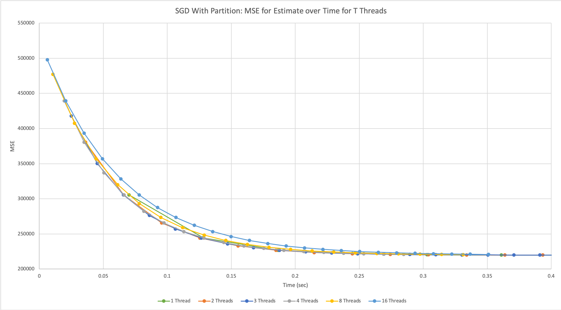
Figure 7: Plot of mean-squared-error over time using alternative SGD design with T = {1, 2, 3, 4, 8, 16} threads run on NVIDIA GeForce GTX 1080 GPU.

In the graph above, multiple threads have a slightly better performance than the sequential implementation, and as the number of threads increased it eventually plateaued as well. The performance was limited mainly by the design of our algorithm. Because as the number of threads increases, each thread receives a smaller and smaller subset of the data, it is not likely that training the model on fewer points would result in an accurate estimate representative of the entire dataset. This presents a cost-performance tradeoff because even though each thread can now compute their subset of the data faster since they receive fewer points, each thread would also compute a less accurate estimate for the same reason.

Conclusion

From our results across both architectures above, we concluded that none of our designs scaled with the number of processors used. While we observed faster convergence rates for a small number of additional processors, each of the designs reached a limit to their performance after around 8 or 16 threads. Therefore, we were unable to take advantage of the high division of labor that the GPU architecture had to offer. Instead, for our designs, it proved better to utilize the computational power and higher clock rate of the Xeon Phi machines to better optimize the performance and accuracy of our gradient descent.

Credit

We both did 50% each

References

Parallelized Stochastic Gradient Descent by Li, Smola, Weimer, and Zinkevich http://martin.zinkevich.org/publications/nips2010.pdf
Stochastic Gradient Descent on Highly-Parallel Architectures by Ma, Rusu, and Torres https://arxiv.org/pdf/1802.08800.pdf

Checkpoint Report

What We’ve Done:

We decided to start our project by applying gradient descent on a linear regression application. We started out by following the tutorial listed below to get a sequential version of batch gradient descent working.

https://spin.atomicobject.com/2014/06/24/gradient-descent-linear-regression/

The tutorial includes a reference implementation in Python and some of their results with a simple data set with 100 points. We implemented this code 3 times. Once in normal C++ for reference, once with CUDA, and once with the OpenMP framework. In addition to just batch gradient descent, we also implemented stochastic gradient descent in all three frameworks as well.
Here a brief description of what the code does. Given a set of N data points of the form (x, f(x)), we try to find a linear function of the form f’(x) = b1 x + b0 to best fit the data. In order to measure fit, we use the error function e =(1/N) Sum [f’(x) - f(x)]^2 over data points. Based on this, we update both b1 and b0according to their partial derivatives on e. Our program updates the parameters for a given number of iterations.

We were able to improve the speedup of batch gradient descent using OpenMP by offloading the work onto the Xeon Phi and utilizing the scheduling of pragma loops. In terms of stochastic gradient descent, since it randomly selects points from the data set, we were able to improve correctness by running this process in parallel and averaging the results. In another design implementation, we were able to build upon this model and also have each process randomly select multiple points to update in each iteration.

Preliminary Results:

In order to test correctness, we first loaded the data set into R in order to visualize the points and find the optimal linear model based on the error function. This served as a baseline. Our linear fit in R yielded the equation y=1.32x + 7.99, with a mean squared error of 110.2574. For our implementations of the program, we were able to get consistent results from both forms of gradient descent when run for enough iterations. Additionally, we tuned our hyperparameters to get our models to converge to a MSE of 112.61 for batch gradient descent with 1000 iterations and a learning rate of 0.0001. Using the same hyperparameters, we achieved an MSE of 113.87 with stochastic gradient descent. Because our data was fairly off center and our parameters, 0and 1, were initialized to 0, a small learning rate and large number of iterations were required for our model to converge on the dataset.

For our intial design for parallelism in stochastic gradient descent, each processor updated its model using random points in all the iterations and averaged the results to improve correctness. Consequently, our results supported this improvement as our MSE consistently decreased as the number of processors increased, while the computation time increased since more synchronization would be needed to average the results.

Goals and Deliverables:

We were able to implement and refine two of our designs outlined in the initial project proposal as restated below: Load all the data on each core, compute the updated value in parallel based on a random data point on each core, and average their results to achieve better correctness. The same as method 1, but compute k updates together on each core and then average their results.

We were able to try out these 2 designs in OpenMP first instead of using GPU programming like our initial project schedule specified. This is because with the basic implementations of batch and stochastic gradient descent there isn’t too much naturally parallel parts of the code, so having a large number of threads isn’t too interesting. We look forward to using the architecture when we come up with our own implementations of a mixed batch/stochastic design to try to optimize correctness as well as performance. Furthermore, with respect to obtaining measurements based on the different approximation algorithms, this deliverable will be pushed back for another couple weeks. This is because we want to come up different design implementations before we take measurements.

At the poster session, we will stick to the original plan and present the following graphs.

Speedup vs Number of Threads for each Architecture
Speedup vs Approximation Factor for each Architecture (Speedup of Max threads available to the machine with respect to 1 thread)
Speedup vs Dataset size for each Architecture (Speedup of Max threads available to the machine with respect to 1 thread)

So far we are on track with respect to our schedule. The only thing that has changed is that we switched the CUDA and OpenMP implementations in our schedule because getting setup with the Makefiles and data took longer than expected. The “nice to haves” are still a maybe. We want to focus on actually using the each architecture to its fullest extent rather than adding another implementation to our project. As of right now, we have basic implementations, but more time can definitely be spent optimizing each of those. An updated schedule can be found in the “Updated Schedule” section.

Updated Schedule:

Week of 11/5 - 11/9: Find a couple data sets to test on Get a sequential version of the code working in C/C++

Week of 11/12 - 11/16: Implement Parallel SGD using OpenMP Implement all four algorithmic designs for OpenMP Implement one of the four algorithmic designs in CUDA

Week of 11/19 - 11/23 (Week of Thanksgiving Break): First Half Improve OpenMP implementations speedup by adding optimizations to the code such as using less critical sections and trading off correctness. (Both) Second Half Convert the for loops to while loops so we can get alpha approximations (Shashank) Get measurements on how long it takes to get within α = {1.5, 1.1, 1.01} of the optimal for all implementations we have coded (Sequential and OpenMP) (Kylee).

Week of 11/26 - 11/30: First Half Implement algorithmic designs 1 and 3 for the CUDA version (Shashank) Implement algorithmic designs 1 and 3 for the CUDA version (Kylee)

Second Half Get more data sets and use them to collect more measurements for all the implementations. (Both)

Week of 12/3 - 12/7: Entire Week Work on additional optimizations on each architecture (Both): Are we using our cache correctly? Have we reduced false sharing? Are there faster ways to do partials sums and add the results together? Can we reorganize the data for faster performance on larger datasets? Where can we sacrifice a little correctness for faster performance?

Week of 12/10 - 12/14: Look into OpenCL if time permits or continue working on optimizations of 12/3-12/7 week otherwise.

Concerns:

Due to the nature of Gradient Descent, it is very much a sequential algorithm to parallelizing it can be a little tricky as we trade-off correctness to get some speedup. We believe we can get up to 8x speedup based on the papers we read, but the results may be very data dependent. Thus, the biggest concern at the time is whether we will actually achieve enough speedup. Currently, we are actually observing some slowdown by using more threads. This could be due to caching problems, synchronization overheads, or something else entirely. Either way, this was an unexpected problem we didn’t anticipate, so we might need to spend some additional time focusing on improving the code. A possible fix that we will experiment with is to include padding in our structs to remove false sharing and lower communication times for each processor as the number of threads increases.

Project Proposal

Summary

We are going to create optimized implementations of gradient descent on both GPU and multi-core CPU platforms, and perform a detailed analysis of both systems’ performance characteristics. The GPU implementation will be done using CUDA, where as the multi-core CPU implementation will be done with OpenMP.

Background

Gradient Descent is a technique used to find a minimum using numerical analysis in times where directly computing the minimum analytically is too hard or even infeasible. The idea behind the algorithm is simple. At any given point in time, you determine the effect of modifying your input variable on the cost you are trying to minimize. In the one dimensional case, if increasing the value of your input decreases your cost, then you increase the value of your input by a small step to get you closer to the minimum cost. Generalizing to higher dimensions, the gradient tells you the direction of the greatest increase on your cost function, so we move the input in the opposite direction to hopefully decrease the value of the cost function.

Building on top of this idea, we have two kinds of gradient descent methods. One is called batch gradient descent and the other is stochastic gradient descent. Let’s discuss both. We can imagine we have some regression problem where we are trying to estimate some function f(x). We are given n labeled data points of the form (xi , f(xi)). Our job is to find some estimator, g(x), of the desired function such that we minimize the squared error (f(xi) - g(xi))2. Now in order to find the true gradient of our cost function, we would need to plug in all our points. This is what’s known as batch gradient descent. If n is large, however, this computation can be very expensive especially since at each time step we only make a small modification. Thus, it does not always make sense to doing such a heavy computation to make a tiny step forward. In contrast, stochastic gradient descent chooses a random data point to determine the gradient. This gradient is much noisier since it doesn’t have the whole picture, but it can greatly speed-up performance. In most cases, it is best to start with stochastic gradient descent, but then eventually switch to batch for fine-grained movement.

As you might observe, the initial position start state may affect our answer when performing gradient descent. This is because the gradient is different at each point and thus starting at a different point may take us in a different direction. With respect to stochastic and batch gradient descent, stochastic gradient has the property that it might jump out of local minima because it has a random aspect to it that makes the gradient more noisy. This has a variety of applications in machine learning where we are working with large data sets and a gradient descent becomes very computationally intensive.

Challenges

The challenges are more related to finding the best suited programming model given an architecture. This is because each architecture calls for a different implementation. With the high number of threads available to GPUs, we can potentially calculate the gradient with a larger number of points and make a more accurate step towards the optimal, but each update may be slower than on multi-core CPUs. In contrast, multi-core CPUs will have the advantage of making updates faster because there is no offload overhead involved. This tradeoff between correctness and speed presents an interesting challenge of finding the programming model that optimizes performance in each case.

Another challenge of the project comes from the fact that we are working with large datasets, so how we organize our memory to hold all the data will be another area of focus for this project. For example, previous papers have stated that it may be beneficial to partition the data into disjoint subsets so each core or block on the GPU doesn’t have to share data. Of course, this may lead to less accurate updates since each core or block only has a part of the whole picture. However, the speedup gained from less sharing might still allow us to arrive closer to the optimal sooner.

Resources

We will start off by implementing our gradient descent using CUDA on NVIDIA GeForce GTX 1080 GPUs and using OpenMP on Xeon Phi Machines. We will start the code from scratch since the actual implementation of the gradient descent isn’t too complex and we may make several modifications to it based on the architecture. This assignment is an exploration of different system designs and architectures, therefore it does not make sense to build off someone else’s code. We want full control of everything.

There are several online papers about this topic. For now, we will use the following two papers for reference.

The one thing we still have to figure out is how to obtain a good dataset. We want a data set that is large and minimizes a non-convex function, so we can observe cases where our gradient descent might fall into a local minimum as opposed to a global one. If time permits, we might run our program on other machines and measure performance on those as well.

Goals & Deliverables

Our overall goal that we plan to achieve is to recreate the results of the papers mentioned above. The desired output of our program is a α = {1.5, 1.1, 1.01} approximation of the optimal solution and we want to examine the runtime it takes to get to those levels of correctness. We aim for a runtime that is around 8x faster than the serial version. We chose this benchmark after reading the papers linked above. According to their results, they achieved approximately a 12x speedup for their data set, so we expect to see similar results.

Over the course of the project, we plan to implement a parallelized version of SGD on both GPUs using CUDA and multi-core CPUs using OpenMP and/or OpenMPI. On both architectures, we want to try a couple of designs. Listed are some of those designs:

Load all the data on each core, compute the updated value in parallel based on a random data point on each core, and average their results to achieve better correctness.
Partition the inputs, compute the updated value for each of the subsets in parallel, and average their results to achieve better correctness.
The same as method 1, but compute k updates together on each core and then average their results.
The same as method 2, but compute k updates together on each core and then average their results.

For the poster presentation, we expect to have lots of graphs of our results. Specifically, we want to at least have the following graphs:

Speedup vs Number of Threads for each Architecture
Speedup vs Approximation Factor for each Architecture (Speedup of Max threads available to the machine with respect to 1 thread)
Speedup vs Dataset size for each Architecture (Speedup of Max threads available to the machine with respect to 1 thread)

If time permits, we also have some additional ideas that we could explore further. We can implement a mixture of batch and stochastic gradient descent to achieve a performance as good or better than the reference papers for some approximation of the optimal. In addition, we can look into OpenCL in order to run SGD on heterogeneous machines that have access to both GPUs and CPUs and measure performance there.

Platform Choice

The goal of this project is to determine the performance tradeoffs of paralleling gradient descent on GPUs and CPUs. The reason we choose to work with NVIDIA GeForce GTX 1080 GPUs and Xeon Phi Machines is mainly because we are most familiar with the machines.

Schedule

Week of 11/5 - 11/9:

Find a couple data sets to test on
Get a sequential version of the code working in C/C++
Get measurements on how long it takes to get within α = {1.5, 1.1, 1.01} of the optimal.

Week of 11/12 - 11/16:

Implement Parallel SGD using CUDA
Implement all four algorithmic designs
Get measurements on how long it takes to get within α = {1.5, 1.1, 1.01} of the optimal.

Week of 11/19 - 11/23 (Week of Thanksgiving Break):

Implement Parallel SGD using OpenMP and/or OpenMPI with just one of the four algorithmic designs discussed

Week of 11/26 - 11/30:

Implement all four algorithmic designs for the OpenMP version
Get measurements on how long it takes to get within α = {1.5, 1.1, 1.01} of the optimal.

Week of 12/3 - 12/7:

Look into additional optimizations that can be done in each architecture in terms of how the data is organized/cached and make those optimizations

Week of 12/10 - 12/14:

Look into OpenCL if time permits or continue working on any of the previous tasks if behind.